When the Spot Moves, What Moved With It? Building a Source Stability Observer

The Question Behind the Project

An inconsistent X-ray spot can be one of those problems where every subsystem looks plausible. The high-voltage output may be moving. Emission current may be changing. A ground-return path may be appearing. Temperature or vacuum may be drifting. The cable may be intermittent. The optics may have moved. The spot-fitting routine itself may simply have produced a bad measurement.

Looking at those signals one at a time is rarely enough. Even plotting them on the same screen is not enough if they were acquired on different timebases or belong to different detector exposures. The useful question is narrower: when the measured spot became unstable, which synchronized measurement changed with it?

I built the Source Stability Observer to answer that question. It is deliberately read-only. It does not command high voltage, regulate the source, or sit in an interlock chain. Its job is to turn a broad troubleshooting problem into a shorter list of experiments worth running next.

Why Time Alignment Comes First

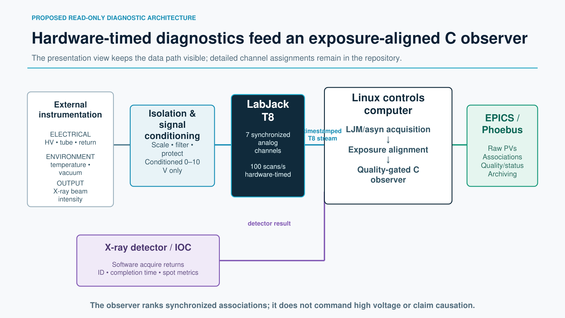
The proposed measurement front end uses a LabJack T8 to stream eight simultaneously sampled analog channels. Those channels can represent conditioned monitor signals such as measured high voltage, tube current, return-current or leakage proxy, filament current, source temperature, vacuum, and X-ray flux. The detector follows a different path and returns an image, completion time, and fitted spot metrics.

That creates a synchronization problem. A simultaneous ADC cannot make an asynchronously acquired image simultaneous. The software therefore creates an exposure ID when an acquisition is requested, retains timestamped T8 scans in a bounded buffer, and selects the scans that fall inside the detector exposure window. It then checks coverage, sample count, timestamp gaps, and numeric validity before producing one aligned record.

In the current architecture, the exposure ID is Linux-side metadata and the alignment uses a common monotonic timebase. If the real detector and source require tighter timing, the right next step is a shared hardware marker whose latency and jitter can be measured. That is a deployment decision, not something I wanted the demonstrator to quietly pretend it had already solved.

Bad Data Does Not Get a Vote

Once the signals are aligned, the next temptation is to calculate correlations immediately. I think that is backwards. The first responsibility of the observer is to decide whether the record is good enough to enter the history at all.

The C quality gate rejects records with invalid upstream quality, incomplete exposure timing, non-finite values, non-positive spot widths, or a spot-fit R-squared below the configured minimum. Rejected samples increment a counter but never enter the rolling window. That detail matters: one saturated or badly fitted image should not skew the mean, inflate the coefficient of variation, and manufacture a convincing-looking correlation from bad evidence.

I used fixed-size state rather than an ever-growing history. The observer has no heap allocation, recursion, global mutable state, blocking I/O, or unbounded work in its update path. The default window is 64 accepted exposures, which is long enough to identify a repeatable signature in the demonstrator while keeping the computation and memory use predictable.

What the Observer Actually Calculates

For each accepted exposure, the code combines the horizontal and vertical spot widths into one spot metric. Across the rolling window it calculates the coefficient of variation (CV), which expresses the spot's standard deviation relative to its mean. CV is useful here because it measures relative instability rather than confusing a larger nominal spot with a less stable one.

Only after the spot CV exceeds its configured limit does the observer evaluate diagnostic branches. It calculates numerically stable Pearson associations between the spot metric and return-current residual, tube current, high-voltage error, and source temperature. High-voltage error is intentional: the interesting quantity is the movement away from the command, not the absolute operating voltage.

The flags are not mutually exclusive, because real faults do not have to arrive one at a time. If the spot is unstable but none of the instrumented domains crosses its association threshold, the observer routes the event toward the optical, mechanical, or estimator branch. It does not label the event “solved” simply because the electrical signals were quiet.

Association Is Not Causation

This distinction is the center of the project. Suppose spot width and return current rise and fall together. That makes the grounding, cable, or insulation path worth investigating. It does not prove that leakage caused the spot change. Both signals could be responding to a third condition, or the timing could still contain an unmeasured bias.

The observer therefore produces a test lead. Causation requires a controlled, repeatable intervention: remove or alter the suspected condition, reproduce the operating state, and verify that the spot response follows. Correlation reduces the search space; the next experiment establishes whether the association means what we think it means.

Using a Digital Twin to Test the Diagnostic Logic

I did not have to wait for a complete physical installation to test the architecture. The repository includes deterministic Python stimulus for normal operation, leakage, emission instability, kV ripple, thermal drift, intermittent cable behavior, optical or mechanical motion, and a deliberately bad image. Each mode is an injected verification condition with an expected observer response.

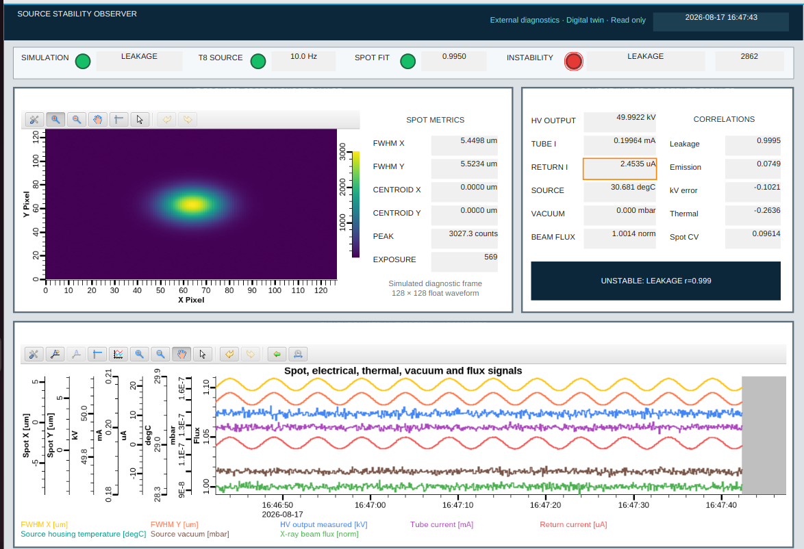
This is where a digital twin is especially useful. I know what disturbance was injected, so I can test whether the quality gate rejects what it should, whether the correct association rises above threshold, and whether competing associations remain low. Fixed-seed scenarios and automated C tests make those results repeatable. The EPICS PV model and Phoebus display then exercise the same operator interface the deployed system would use.

Why C, EPICS, and Phoebus

I kept the analytics, quality gate, exposure synchronizer, and LabJack acquisition boundary in C. That makes the decision path portable, bounded, and testable without requiring EPICS, a GUI, or even the physical T8. Python is used to generate deterministic stimulus for the present demonstration; it is not intended to become the production acquisition or analysis engine.

EPICS provides the operational contract around that core: named process variables, engineering units, alarm states, heartbeat, counters, observer results, and an image waveform. Phoebus provides the operator view. In a physical deployment, a C++ asynPortDriver wrapper would own the worker thread around the C LabJack adapter because that EPICS interface is class-based.

This separation was intentional. Acquisition can change without rewriting the statistics. The display can change without changing the observer. The simulator can be replaced by real equipment while preserving the PV contract. More importantly, each boundary can be tested on its own.

What Is Demonstrated, and What Is Not

The repository contains a working C observer, exposure synchronizer, defensive LJM acquisition adapter, tests, EPICS database, Python simulator, Phoebus display, installation scripts, and documentation. It demonstrates that the proposed interfaces and diagnostic logic can be exercised repeatably without hardware.

It is not yet qualified for machine operation. Physical deployment still requires verification of monitor-output ranges, isolation, signal conditioning, grounding, calibration, bandwidth, detector integration, timing uncertainty, reconnect behavior, stream backlog, long-duration reliability, and the real equipment's safety procedures. The LabJack must only see approved, conditioned low-voltage outputs; it is never connected directly to a high-voltage node.

I think stating that boundary makes the project stronger. A useful demonstrator should prove what it can and make the unfinished engineering visible. Otherwise, a polished screen can create more confidence than the evidence supports.

The Broader Lesson

Troubleshooting often fails because the data exists but the context connecting it does not. Signals are logged at different rates, timestamps mean different things, poor measurements are allowed into the history, and then a plot is expected to explain the machine after the fact.

The Source Stability Observer reverses that order. Define the exposure. Align the evidence. Reject the bad records. Measure the instability. Rank the associated domains. Then design the experiment that can establish cause. That sequence is useful well beyond X-ray sources; it applies anywhere a performance symptom sits downstream of several plausible physical systems.

The complete source code, tests, display, diagrams, and deployment notes are public on GitHub for technical review.

Rob Rainer is a controls and systems engineering leader with more than 20 years of experience across materials science, particle accelerators, precision instrumentation, distributed control systems, electrical engineering, operations, and technical leadership. He spent over 15 years at Brookhaven National Laboratory's NSLS-II, including as Senior Technology Engineer and Lead Operator.

← Back to Articles